
This blog presents two methods for estimating Player xG
- Method 1 – First Principles from Match xG
- Method 2 – Benchmarking against market information
Goalscorer markets can be highly volatile

Volatile markets can lead to edges if we have confidence in our numbers. To estimate value in Player Goalscorer markets we benefit from estimating the expected goals a Player will have in a game (Player xG). Player xG can be extrapolated to the probability of a player scoring 1 goal, 2+ goals, 3+ goals, a goal in each half, first goalscorer and a range of Player markets.
Method 1 – First Principles from Match xG
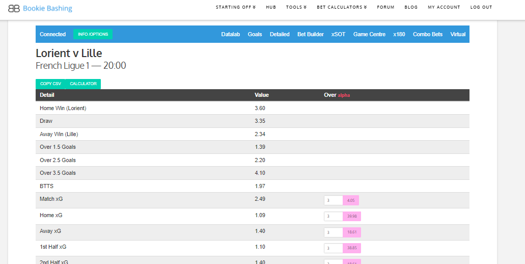
We start with the expected goals in a match:
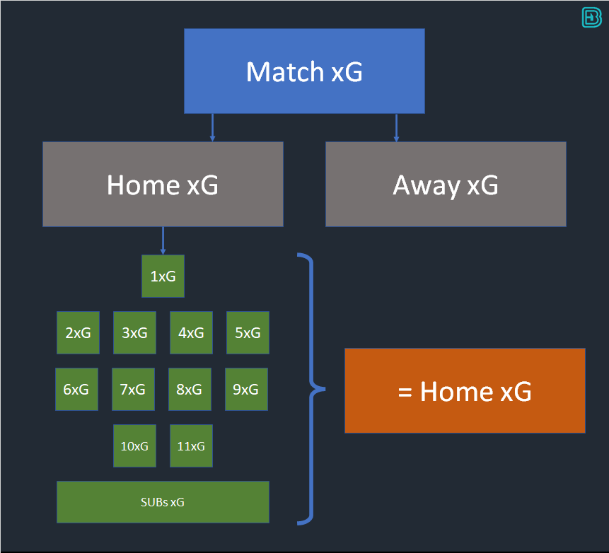
There is a direct relationship between the Team xG and the probability of a player scoring. The odds of a player scoring are higher in low scoring matches than they are for the same player in a high scoring match. There can only be a finite number of goals in a match, and this has a direct relationship on the xG of each player on the pitch. The sum of the xG of the Starting XI + Subs = the Team xG.
We assume Team xG exists as an input to our problem.
(Match xG can be estimated through a number of different methodologies. At bookiebashing.net we have a tool that calculates the xG for every game in the primary leagues from market conditions. Match xG can be split into Home xG and Away xG through a number of methodologies – e.g. a function of the match odds. At bookiebashing we provide the home and away xG for each game, hence why we presume Team xG exists as an input to our problem)
The Team xG needs to be split between the potential scorers on the pitch, Starting XI and potential substitutes aswell.
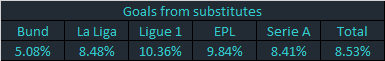
Historically, 8.5% of goals have been scored by substitutes in the top European leagues (from a sample of games where players have scored 6 or more goals of the season). We can use this as an empirical function and assume that the Starting XI will account for 91.5% of the Team xG.
There are plenty of useful online sources for predicted line-ups, like whoscored.com
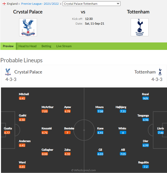
To distribute the 91.5% of team xG amongst the players we can work out the historical goals/game of each player to give a score rate. We can then normalise the score rate amongst the Starting XI to give a % distribution of goals in the team that sums to 1 (this is a simplified methodology. Additional information, such as starting formation, will have an affect on the distribution of goals amongst a team. If Harry Kane is starting at left back, he’s getting fewer goals than if he starts up front).
Example
Lets assume the XI Players in our home team above have the following historical score rates:
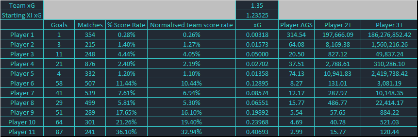
We can take the score rate, and apply the following methodology to work out the AGS odds of each player:
- Normalise the score rate so that the sum equals 1 across all XI players
- Determine the starting XI xG by taking the team xG and multiplying this by 0.915
- Distribute the starting XI xG amongst the players by a function of their normalised team score rate
- Use a Poisson distribution to determine Player AGS: in excel “AGS = 1-(poisson.dist(over, xG, true))^-1”
- We can also use a Poisson distribution to estimate the probability of the Player score 2 and 3 goals.
If we have the probability of all 22 player scoring in the match, we can run a Monte Carlo simulation to determine Player FGS price.
Method 2 – Inverse Poisson from market information
Instead of starting with Team xG we can start with Player AGS from an unbiased source.
An alternative methodology bypasses these issues – using market information and applying an Inverse Poisson relationship.
Player AGS can be worked out from the application of a Poisson probability distribution using Player xG. The reverse is also true – we can use an unbiased Player AGS price and apply an inverse Poisson relationship to estimate the mean Player xG the market maker has used in their modelling.
Whilst this doesn’t help us extrapolate a price for Player AGS (we use this as a starting input), it does help us extrapolate a price for Player 2+, Player 3+, Player to Score in Both Halves.
The Poisson distribution equation:
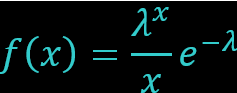
- where f(x) = the probability (e.g. AGS odds)
- λ = the mean (e.g. Player xG)
- x = the number of occurrences (e.g. Over 2 = Hattrick)
To calculate the mean λ from the odds “f(x)” we must rearrange and solve the equation for λ.
We have a number of options for benchmarking a fair price for AGS. The back, lay, LPM and midpoint on the exchange are options, as is using the top bookmaker price with an appropriate markup.
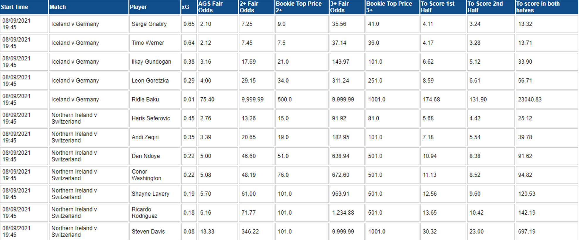
We are trialling a methodology at BB monitoring the live trading prices for AGS on Betfair exchange for all matches in a day. By applying an inverse Poisson relationship to the AGS price, we can estimate xG. From the xG, we can extrapolate forwards to 2+ and 3+ goals.
We can then target these markets at scale on the bookmaker and at the exchange to find value, especially when smart money results in a player steaming in.
NB Its worth noting that 2+ goals tends to fit a Poisson relationship between AGS and 2+ on the exchange.
NB 3+ goals (i.e. Player to score a Hattrick) tends to trade at a slightly lower price than Poisson (over 2 goals, xG). This could be because of influence from a concept such as dominance in a game (where if a player scores 2 goals they are more likely to score a 3rd) or it may be because layers are taking advantage and offering value to recreational backers in an illiquid market.