
Multi-Attribute Decision Analysis
Multi-attribute Decision Analysis (MADA) is a sub discipline of mathematical science that applies advanced analytical methods to improve decision making. MADA employs techniques such as modelling, statistics, optimisation and operations research to arrive at optimal or near-optimal solutions to complex decision making problems.
MADA involves the following steps:
- Identify the metrics relevant to the problem at hand
- Weight the metrics in terms of how important they are to the overall solution
- Identify all possible mathematical solutions
- Determine the metric scores for each solution
- Apply one of the MADA frameworks to determine near-optimal solutions.
The Efficiency Frontier and Betting
In portfoilio theory the efficiency frontier is the set of solutions that occupies the “efficient” part of the risk-return spectrum. In Step (5) above we reference that a MADA will return near-optimal solutions. The objective is to determine each solution that lies on the efficiency frontier. In golf betting we can apply the same mathematical framework. A golf tournament may have over 160 competitors. It is technically possible to search for the “optimal solution” – the single golfer who is presents the most attractive betting proposition. However the odds in a golf field may range from 10/1 up to 1000/1. Many golfers win with pre-tournament probabilities of less than 0.01. Rather than choose a single optimal solution it may be more comfortable (under variance) to select a portfolio of golfers for each tournament.
Our problem now becomes a search for the “efficiency frontier” in a golf tournament field. We want to search for the set of golfers that occupy the efficient part of a risk-return spectrum.
Golf Betting
Professional golf betting (on the outright market) involves the determination of bookmaker or exchange prices where the price available exceeds a utility price as set by our own analytics. If we can estimate a “fair probability” for each player in a market that sums to 100% then the objective is to find a price at the bookmaker that exceeds our estimation of the “fair probability”.
Each player in a golf tournament is priced up relative to every other player winning. It is important to estimate the strengths of each individual player – but is arguably more important to work on the analytical framework that compares the strength of each player relative to every other player in the field.
Golf Metrics
Golf data providers collect information on a wide range of metrics on player performance such as:
- Greens in Regulation (Benefit)
- Bogey Scoring (Cost)
- Driving Accuracy (Benefit)
- Driving Distance (Benefit)
- Putts per round (Cost)
- Recent Birdies (Benefit)
- Recent Eagles (Benefit)
- Scrambling (Benefit)
- SG: Approach the Green (Benefit)
- SG: Around the Green (Benefit)
- SG: Off the Tee (Benefit)
- SG: Putting (Benefit)
- SG: Tee-To-Green (Benefit)
It is possible to match up certain metrics with various courses. For example a course such as Augusta places a high emphasis on putting skills. A links golf course on the coast of Scotland will usually reward driving accuracy.
Various services (such as fantasylabs) can help us determine metrics that would have trended towards predicting which golfers performed over expectation in historical events. We can use these services to determine a shortlist of metrics from which we can apply an analytical MADA to the field.
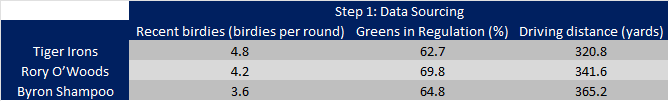
Data Sourcing
In MADA we have i attributes and j alternative solutions. Imagine we are gathering data for the the Open Championship at St Andrews. By looking at this tournament and golf course we determine that recent birdies, greens in regulation and driving accuracy are all attributes that have been historical indicators that could predict success.
To simplify the problem we are going to look at a field of just 3 players:
- i = 3
- j = 3
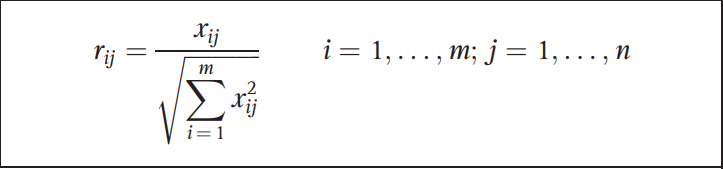
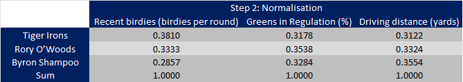
Normalisation
These metrics are incommensurable (meaning they have no common standard of measurement). We are comparing units of “birdies per round”, “%s” and “yards”. To account for this we can calculate a normalised score (r) by dividing the observation (x) by the sum of all observations for each attribute. The normalised score (r) can be worked out by
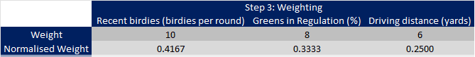
Weighting
We can weight the three attributes to apply a relative importance to one attribute over another. There are various methodologies in literature for weighting attributes, such as the pairwise comparison technique. We will keep it simple for this blog and subjectively score the importance of each attribute out of 10.
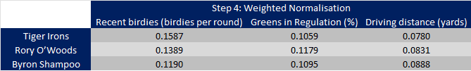
Weighted Normalisation
Every observation can be multiplied through their relevant attribute weight to determine a weighted, normalised score for each attribute. This accounts for the importance of each metric. The weighted, normalised score (v) is calculated by:

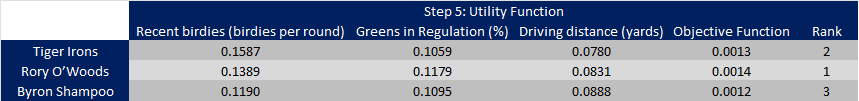
Utility Function
The identification of a weighted, normalised score for each attribute allows us to combine the scores into a single Utility Function. The Utility Function is a utility score which we can use to rank the attractiveness of each player under the decision attributes and applied weighting. There are many different techniques for combining scores into an utility function. The technique below takes the product of the set of weighted, normalised scores for each player. We can then rank each player by a magnitude of their utility function.
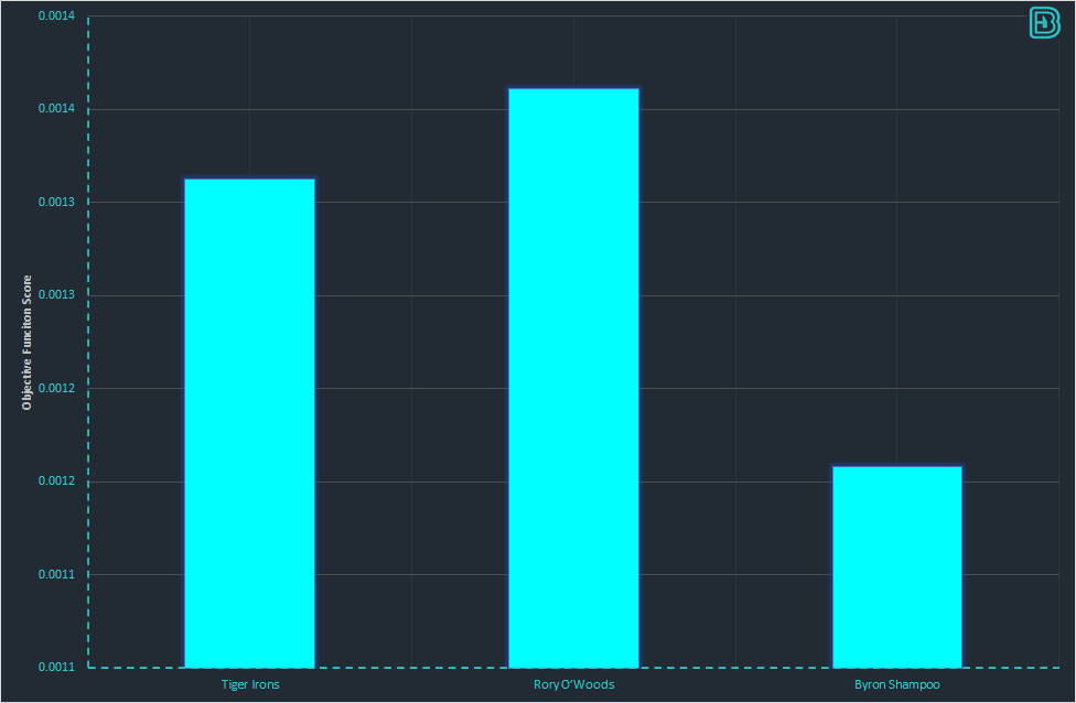
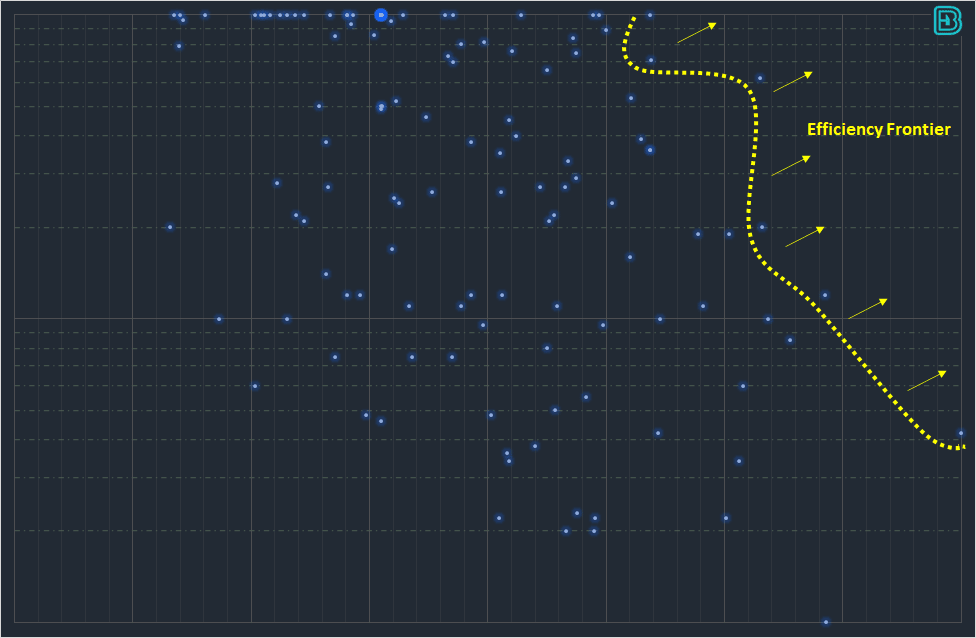
Efficiency Frontier
The score in the graph above does not assist us completely with our betting. We see that Rory O’Woods has the best score, but to bet we need to know what the odds are. If he is 1/100 then he is unlikely to be a value bet, regardless of how well he scores under Multi-Attribute Decision Making.
To aid us with our golf betting we can plot a graph that shows the MCDM utility score vs the odds available:
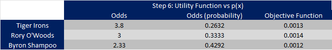
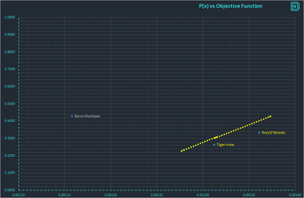
Both “higher utility function” and “higher odds” are benefit constraints (the higher the position on the axis the more attractive the solution). In this graph we can see that the efficiency frontier consists of two points. Byron Shampoo is is not on the efficiency frontier – we can get a higher score than Rory for higher odds. Both of these attributes are attractive, and therefore there is no logical reason to choose Byron over Rory or Tiger. We cannot immediately choose between Tiger and Rory – they are both near-optimal solutions and both sit on the efficiency frontier.
Now that we have identified the players on the efficiency frontier we know who we will not be betting on (Byron Shampoo). The selection of either Rory or Tiger (or both player) is now a personal choice associated with our risk profile. What variance do we want to bet to? Do we want to cover 30% or 50% of the field? Do we prefer a higher probability of success with a lower utility function, or a lower probability of success with a higher utility function?
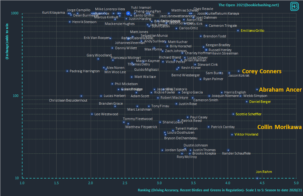
Real world example – The Open 2021
The graph below shows a Multi-Attribute Decision Making plot for the Open Championship 2021 at the Royal St Georges Golf Course. Through a review of the tournament we identified that Driving Accuracy, Recent Birdies and Greens in Regulation were attributes that were relevant. We obtained the scores for all 156 players and then weighted the attributes as:
- Driving Accuracy 10/10
- Recent Birdies 8/10
- Greens in Regulation 6/10
Through a Multi-Attribute Decision Analysis we scored every player with a utility function. The score was adjusted to fit every player into a rank of 1 to 5. By obtaining the odds for the tournament we were able to plot the following graph:
We can identify an efficiency frontier with six golfers on it:
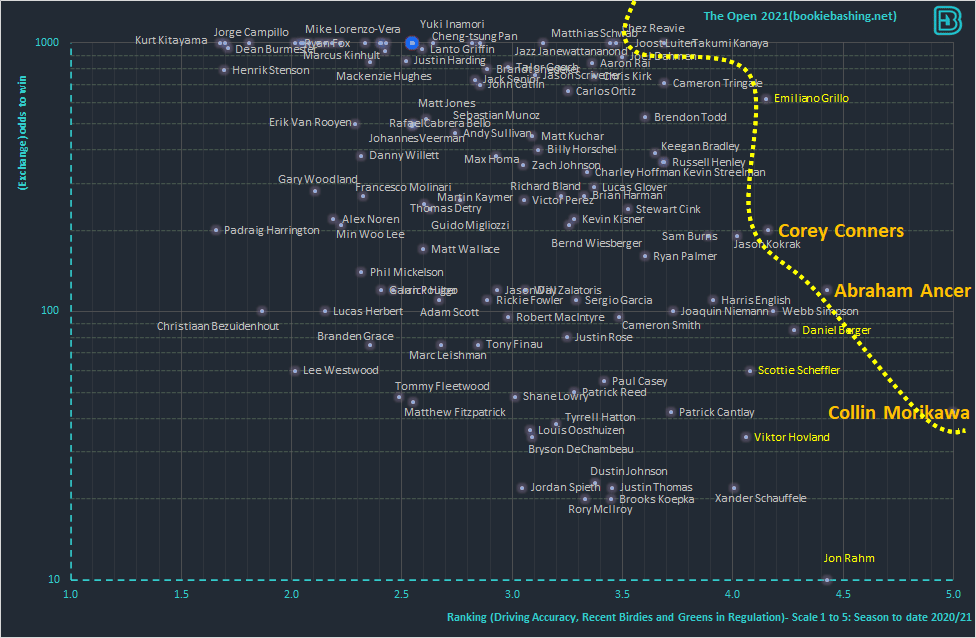
Takumi Kanaya, Cameron Tringale, Corey Conners, Abraham Ancer and Morikawa all sat on the efficiency frontier. No golfer has both a higher score and a higher price than these six golfers.
We posted the graph above on the Wednesday before the Open in July 2021. We highlighted 8 golfers through an assessment of
- How close to the efficiency frontier are they?
- How low are their odds?
A golf betting strategy may choose to take golfers at 1000/1 – however one hundred golfers at 1000/1 is still only 1% of the field win probability coverage. We would need to wait a long time for a winner. There is a tradeoff with lower priced golfers in the field; the lower priced golfers may not have a utility score as high, but their low price means that (in principle) an odds compiler sees something that we may not be, and that the the variance of betting on these golfers will be flatter. This needs to be factored in to the decision making process and it is often attractive to bet on golfers outside of the efficiency frontier but with a relatively high utility function score in comparison to other players in their price range.
156 players finished in the leaderboard. How did the golfers in our analysis fair? It could be argued that they performed beyond an expectation from purely looking at the markets:
- 1st Colin Morikawa (42.0)
- 3rd Jon Rahm (9.4)
- 8th Daniel Berger (85.0)
- 8th Scottie Scheffler (60.0)
- 12th Emilliano Grillo (620.0)
- 12th Viktor Hovland (34.0)
- 15th Corey Conners (200.0)
- 59th Abraham Ancer (120.0)