
Below we present three methods for estimating over x goals in y games:
- Method A – using the exchange Daily Goals Market
- Method B – using over 0.5 to over 7.5 exchange data for each game
- Method C – using a discrete probability distribution
This is followed by a case study using real data and compare the results of each Method.
Bookmakers often offer a bet “over x goals in y games”.

Method A – using the exchange Daily Goals Market:
This method is clearly cheating as we rely on others to work out the maths and the wisdom of the crowds to form a price. It is the easiest method to use when it is available – when (on rare occasions) the set of “y games” has an associated market on the exchange. In this instance the lay price, the middle of the gap and the last traded price are all viable options for benchmarking the probability. This market is not the most liquid, so attention should be paid on reasons for it to be inefficient (e.g. the presence of boosts on particular lines).

Method B – using over 0.5 to over 7.5 exchange data for each game.
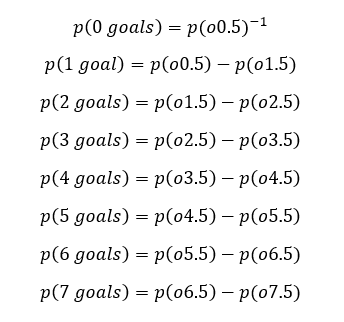
We can use over 0.5 to over 7.5 exchange data to approximate the odds of exactly 0 to 7 goals in each game. We assume that the odds of 8+ goals are negligible and discount them for our calculations (only 12 of 12,984 UK matches between 2012 and 2019 finished with 8 or more goals).
For any game
The o2.5 market is liquid for a large number of games on the exchange. The other o/u goals markets are not as efficient; however we can use a large set of historical data to populate these games. The relationship between o2.5 and o0.5 to o7.5 is typically linear as the probability of o2.5 changes. The following graphs show the pre-KO last traded price vs the o2.5 odds of every game on betfair exchange in October 2018:
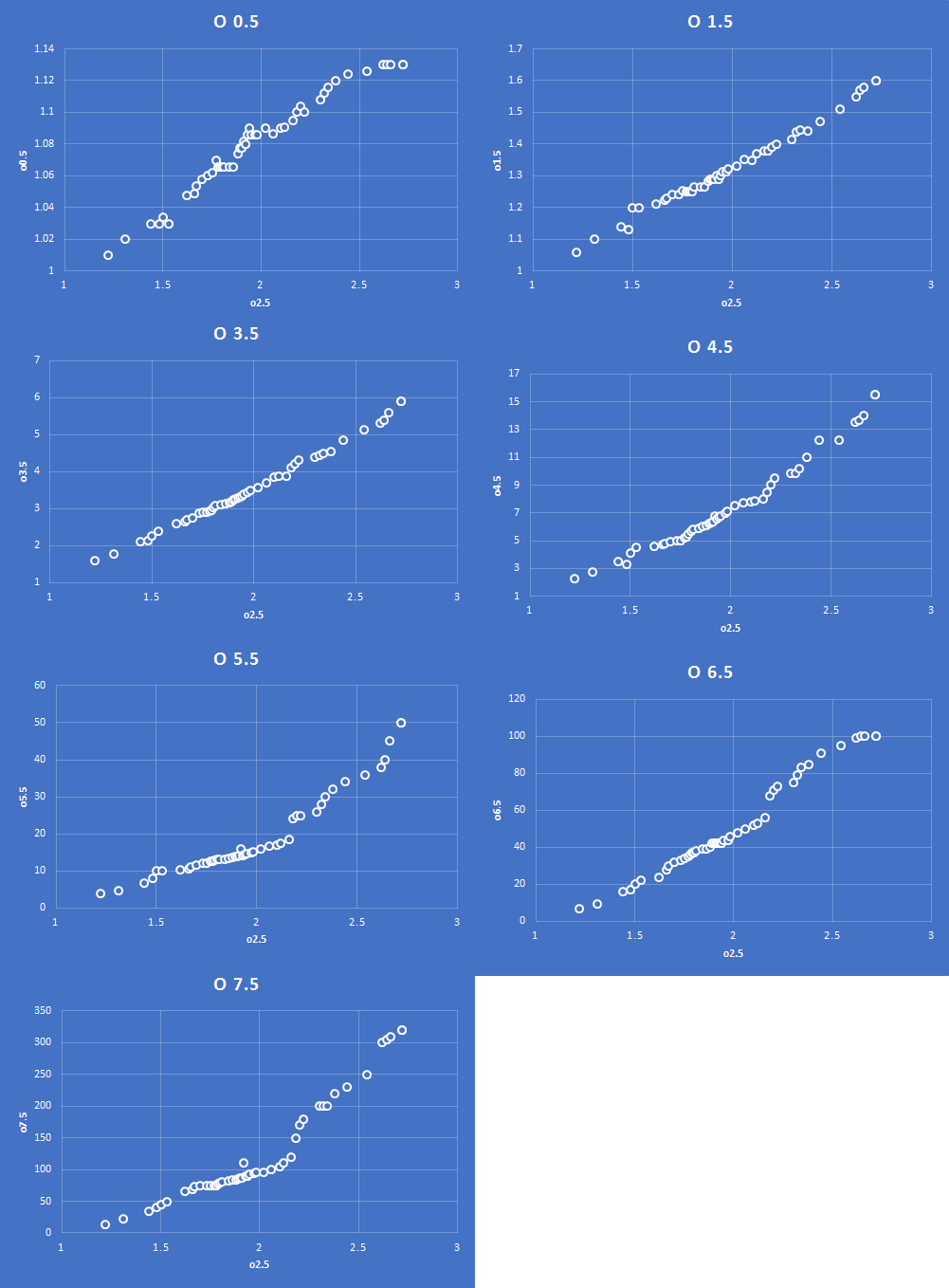
By using this library of probability we can estimate the odds for o0.5, o1.5, o3.5, o4.5, o5.5, o6.5 and o7.5 through an assessment of the available price for o2.5.
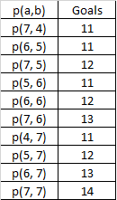
With 2 matches a and b, we can now calculate the probability of every permutation of goals up to 7+7 = 14 goals:
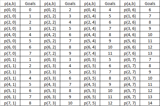
The final step of the process is to sum the relevant probabilities for each over goals calculation. For example, in the above table we would sum the following to approximate “over 10 goals in 2 matches”.
We can repeat this for all permutations for x goals up to y matches. With y matches there are 7^y permutations. This number of solutions quickly becomes very large therefore it is necessary to process this calculation through concise coding.
Method C – Discrete Probability Distribution
We can take the mean expected number of goals in y games and apply it to a discrete probability distribution to calculate the probability of over x goals.
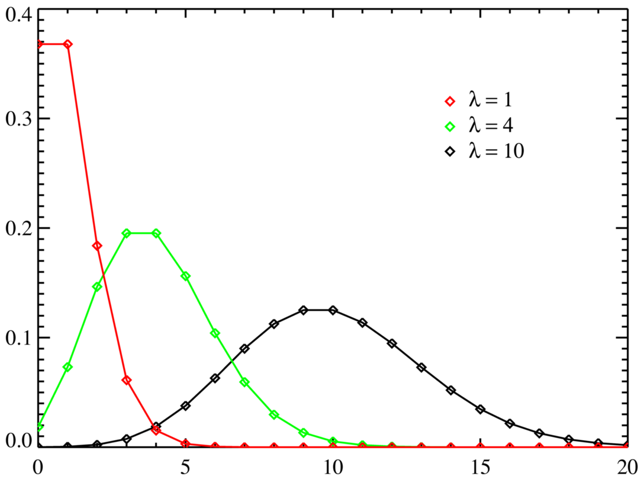
The mean expected number of goals can be taken from the Sell, Buy or midpoint of the Total Goals line at a Spread Site:

The Sell line provides a pessimistic approximation, the buy line provides an optimistic approximation and the midpoint provides an averaged approximation.
A spreadsheet for calculating the Poisson discrete probability distributions given the input of “over x goals” and a mean Total Goals line is available here.
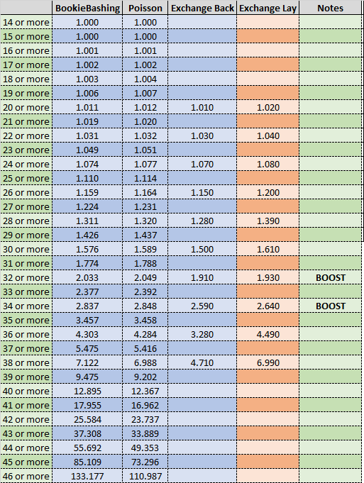
A comparison of the 3 methods
We compared the three techniques using data from the 10 English Premier League games on Sunday 12th May. A market was available for these games on the exchange.
The exchange market was inefficient; there were some gaps between the backs and the lays and there was a relatively low amount of liquidity available. There were also bookmaker boosts on a couple of the prices, which will skew the market with arbitrage players attempting to trade a price.

The table below shows the probability of over 14 goals to over 46 goals using the BookieBashing model based on o2.5 lay data and the Poisson model.
The following graph presents a plot of the probability of over x goals in these 10 games based on the three methodologies above:
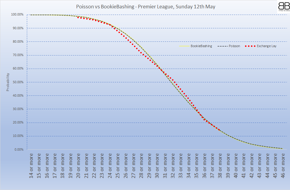
It can be seen that the Bookiebashing (B) and Poisson (C) models result in very similar approximations. The available exchange method (A) provides a skewed approximation, due to the fact that the market was inefficient.